Lognorm Demo ($1848649) · Snippets

Hello,

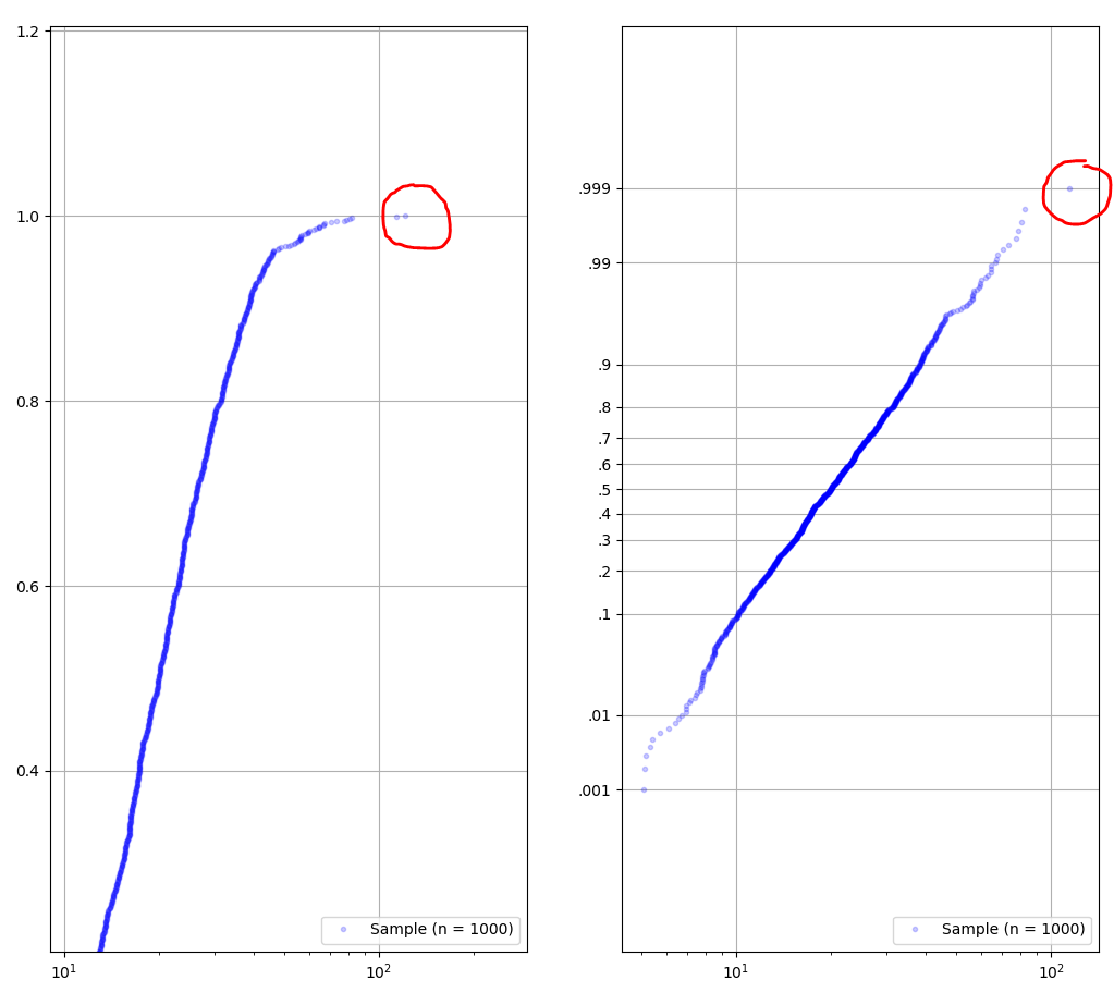
Thanks a lot for this sharing. This seems it is the only example for cdf probability paper plot available on the net. Result is really perfect except but the last sample is not plotted when using set_yscale('ppf').

Do you know if there is a method to plot even the last sample with set_yscale('ppf') ? I would avoid adding an additional fake sample to plot it.

On the right a zoom on the high value of samples without ppf yscale. On the left the plot with ppf scale.

Thanks, Benoit

Hmm, I can confirm your observation but right now have no explanation for it. I'll be travelling for the next 2 weeks and try to have a look at it when I'm back.
Steffen

The plotting position on the probability axis is defined by the inverse of the cumulative distribution function which is + and - infinity for 1 and 0 respectively and therefore can't be shown on the axis. Hence the last value, having a cdf of 1, is missing.
To overcome this situation, different plotting positions were introduced, see the discussion of empirical probabilities estimator versus plotting-position estimator in the Details section here. So in order to show all values we'll have to use a different plotting position the simply i/n, e.g. (i-0.5)/n, i.e. cumprob = ECDF(values)(values) - .5/size instead of cumprob = ECDF(values)(values).

During looking into this I came across mpl-probscale which makes probability scales for matplotlib. So there's basically no need to roll your own as shown in this snippet. It also includes a section on different plotting positions here.

With the new FuncScale of matplotlib 3.1 we can dramatically shorten it for the normal distribution scale. We still need to register a scale class in the case of the lognormal distribution scale as we need to pass the scale parameter s:

import numpy as np
import scipy.stats as stats
from matplotlib import scale as mscale
from matplotlib import transforms as mtransforms
from matplotlib.ticker import FixedLocator, FuncFormatter

class PPFScale(mscale.ScaleBase):
    name = 'ppf'

    def __init__(self, axis, *, s, **kwargs):
        super().__init__(axis)
        self.s = s

    def get_transform(self):
        return self.PPFTransform(self.s)

    def set_default_locators_and_formatters(self, axis):
        axis.set_major_locator(FixedLocator(np.array([.01,.1,.2,.3,.4,.5,.6,.7,.8,.9,.99,.999])))
        axis.set_major_formatter(FuncFormatter(lambda x,_: f'{x}'[1:]))

    def limit_range_for_scale(self, vmin, vmax, minpos):
        return max(vmin, 1e-6), min(vmax, 1-1e-6)

    class PPFTransform(mtransforms.Transform):
        input_dims = output_dims = 1

        def __init__(self, s):
            mtransforms.Transform.__init__(self)
            self.s = s

        def transform_non_affine(self, a):
            return stats.lognorm.ppf(a, s=self.s)

        def inverted(self):
            return PPFScale.IPPFTransform(self.s)

    class IPPFTransform(mtransforms.Transform):
        input_dims = output_dims = 1

        def __init__(self, s):
            mtransforms.Transform.__init__(self)
            self.s = s

        def transform_non_affine(self, a):
            return stats.lognorm.cdf(a, s=self.s)

        def inverted(self):
            return PPFScale.PPFTransform(self.s)

mscale.register_scale(PPFScale)


if __name__ == '__main__':
    import matplotlib.pyplot as plt
    from statsmodels.distributions.empirical_distribution import ECDF, _conf_set
   
    # test data
    size = 1000
    loc = 0
    scale = 20
    s = .5
    
    rv = stats.lognorm(s = s, loc = loc, scale = scale)
    values = rv.rvs(size = size, random_state=1)
    mu = np.mean(np.log(values))
    sigma = np.std(np.log(values))

    # calculate empirical CDF
    values.sort()
    cumprob = ECDF(values)(values)

    # fit data
    sfit, locfit, scalefit = stats.lognorm.fit(values, floc = 0)
    rvfit = stats.lognorm(loc = locfit, scale = scalefit, s = sfit)

    # plot
    plt.rcParams['axes.grid'] = True
    fig, (ax1, ax2, ax3, ax4) = plt.subplots(1, 4)
    fig.suptitle(f'lognormal (loc = 0): scale = {scale:.3f}, s = {s:.3f}\n' 
                 f'sample: exp(mean(ln(x))) = {np.exp(mu):.3f}, std(ln(x)) = {sigma:.3f}    ' 
                 f'fitted: scale = {scalefit:.3f}, s = {sfit:.3f}' )
    x = np.linspace(values.min(),values.max(),100)

    # pdf
    ax1.plot(x, rv.pdf(x), 'r-', label = 'True PDF')
    ax1.hist(values, bins=15, density = True, histtype = 'stepfilled', alpha = 0.2, label = f'Sample (n = {size})' )
    ax1.plot(x, rvfit.pdf(x), 'g-', label = 'Fitted PDF')
    ax1.legend(loc = 'upper right')
    
    # cdf
    ax2.plot(x, rv.cdf(x) ,'r-', label = 'True CDF')
    ax2.step(x, ECDF(values)(x) ,'b-', label = 'Empirical CDF')
    ax2.plot(x, rvfit.cdf(x), 'g-', label = 'Fitted CDF')
    lower, upper = _conf_set(ECDF(values)(x))
    ax2.fill_between(x, upper, lower, alpha = 0.2, label = 'DKW Confidence Band')
    ax2.legend(loc = 'lower right')

    # cdf probability paper normal vs log
    ax3.plot(x, rv.cdf(x) ,'r-', label = 'True CDF')
    ax3.plot(values, cumprob, 'bo', alpha = 0.2, markersize = 3, label = f'Sample (n = {size})' )
    ax3.plot(x, rvfit.cdf(x), 'g-', label='Fitted CDF')
    ax3.set_xscale('log')
    ax3.set_yscale('function', functions=(stats.norm.ppf, stats.norm.cdf))
    ax3.yaxis.set_major_locator(FixedLocator(np.array([.001,.01,.1,.2,.3,.4,.5,.6,.7,.8,.9,.99,.999])))
    ax3.yaxis.set_major_formatter(FuncFormatter(lambda x,_: f'{x}'[1:]))
    ax3.set_ylim(0.0001,0.9999)
    ax3.legend(loc = 'lower right')
    
    # cdf probability paper lognormal vs linear
    ax4.plot(x, rv.cdf(x) ,'r-', label = 'True CDF')
    ax4.plot(values, cumprob, 'bo', alpha = 0.2, markersize = 3, label = f'Sample (n = {size})' )
    ax4.plot(x, rvfit.cdf(x), 'g-', label='Fitted CDF')
    ax4.set_yscale('ppf', s=s)
    ax4.set_ylim(0.0001,0.9995)
    ax4.legend(loc = 'lower right')

    plt.show()